From Datalog to SVG

When working with generative algorithms it is convenient to store the results as you make them. I usually export vector drawings to .svg. This has a few drawbacks. Most notably that the actual graph (topology) is more or less lost in the .svg file. Making it impossible to re-draw an .svg from the graph with modified drawing logic.

I have exported results in different ways over time. Among others to .obj files. The following is the most recent attempt to store results in a more convenient way.

In this post I described my Datalog query language for querying graphs in an in-memory graph data structure (cl-grph). You may want to read that post before moving on. However, the following Datalog examples are pretty simple.

Exporting the Graph

Let's make a graph instance, g, with some random data as an example:

; create a new instance of g, and generate
; some random edges with different properties
(let ((g (grph:make)))
  (grph:modify! (g)
    (loop repeat 20 do
      (rnd:prob 0.4
        ; -> adds edge between two random
        ;    verts with property :pth
        (-> (rnd:rndi 5) (rnd:rndi 5) (list :pth))
        ; <> add edges in both directions with
;    several props: :pth :pth2, (rndprop 10)
        (<> (rnd:rndi 5) (rnd:rndi 5)
            (list :pth :pth2 (rndprop 10))))))

The various edge properties like :pth, :pth2, can be used (among other things) to associate different drawing styles with a set of edges. Further on we use :stipple for stippled edges.

Here is the query to get all combinations of edges and properties we want to export from our graph:

(grph:qry g :select (?p ?x ?y) :where (?x ?p ?y))
;;
;; :PTH[0-9] are the random properties 
;; ((:PTH  0 1) (:PTH  0 3) (:PTH  0 4) (:PTH  1 0) (:PTH  1 4)
;;  (:PTH  2 3) (:PTH  3 2) (:PTH  3 4) (:PTH  4 0) (:PTH  4 1)
;;  (:PTH  4 2) (:PTH  4 3) (:PTH2 0 1) (:PTH2 0 4) (:PTH2 1 0)
;;  (:PTH2 1 4) (:PTH2 2 3) (:PTH2 3 2) (:PTH2 3 4) (:PTH2 4 0)
;;  (:PTH2 4 1) (:PTH2 4 3) (:PTH0 0 1) (:PTH0 1 0) (:PTH0 1 4)
;;  (:PTH0 4 1) (:PTH2 2 3) (:PTH2 3 2) (:PTH3 0 1) (:PTH3 1 0)
;;  (:PTH6 0 1) (:PTH6 1 0) (:PTH8 0 4) (:PTH8 4 0) (:PTH9 3 4)
;;  (:PTH9 4 3))

Variables in the cl-grph Datalog implementation have to be prefixed with ?. So this query can be read as "select all existing combinations of (?p ?x ?y), where there is an edge from ?x to ?y, with property ?p".

You no doubt see that the properties are repeated a lot. A more space efficient export can be achieved using this query instead:

(grph:qry g
  :select (?p (grp ?x ?y)) ; group (?x ?y) for every ?p
  :where (?x ?p ?y)        ; same condition as before
  :collect (list ?p (flatten (grp ?x ?y))))
;;
;; ((:PTH (4 3 4 2 4 1 4 0 3 4 3 2 2 3 1 4 1 0 0 4 0 3 0 1))
;;  (:PTH0 (4 1 1 4 1 0 0 1)) (:PTH3 (1 0 0 1)) (:PTH6 (1 0 0 1))
;;  (:PTH2 (4 3 4 1 4 0 3 4 3 2 2 3 1 4 1 0 0 4 0 1))
;;  (:PTH8 (4 0 0 4)) (:PTH2 (3 2 2 3)) (:PTH9 (4 3 3 4)))

This seems good enough for now. And importing it again is just a matter of reading the data back in, looping over the properties, and adding them to a fresh graph.

Before we export the graph data to file let's look at a different use case for the query language.

Datalog to SVG

While experimenting with the export I decided to make a small DSL for drawing SVGs directly from Datalog queries. I won't go into the DSL in detail here, but you can recognize the Datalog queries pretty easily as they still use the prefixed variables ?x and ?y as we saw above.

Also notice that the DSL uses .& as triggers for symbols to be interpreted in a particular way. Much like the DSL for vector mathematics I described previously.

Here is the code that draws an .svg from Datalog queries, using the new DSL; exports the graph (and spatial data) to a .grph file; and stores the literal code used to draw the .svg alongside the graph data.

; write grph, g, and spatial data, v, to "tmp2"
(grph:write-with-script ("tmp2" g v)
  ; SVG and PRNG instance
  (let ((svg (wsvg:make)) (rs (rnd:make 473)))
    ; initiate DSL context (macro)
    (wsvg/grph:selectors (g v svg)
      ; select all :path edges
      (.&ws ?x ?y (?x :path ?y)
        ; draw all segments
        (.&path :sw 1.75 :so 0.85))
      ; select all :stipple edges
      (.&ws ?x ?y (?x :stipple ?y)
        ; draw stippled segments with prob. 0.7
        (rnd:prob rs 0.7 (.&stip 2f0 1.3 :sw 0.75 :so 0.7)))
      ; select all verts with less
      ; than 3 adjacent verts
      (.&vs ?x (and (or (?x :path ?y) (?y _ ?x))
                    (% <= (grph:edge-count g ?x) 3))
        ; draw circles with 0.1 prob.
        (rnd:prob rs 0.1 (.&circ 8f0 :fill :black :so 0.8 :fo 0.8))))
    (wsvg:save svg :fn))))  ; save svg

In other words the exported .grph file now contains the graph (and spatial) data right next to the logic used to draw it. Including the pseudorandom number generator (PRNG) with appropriate state.

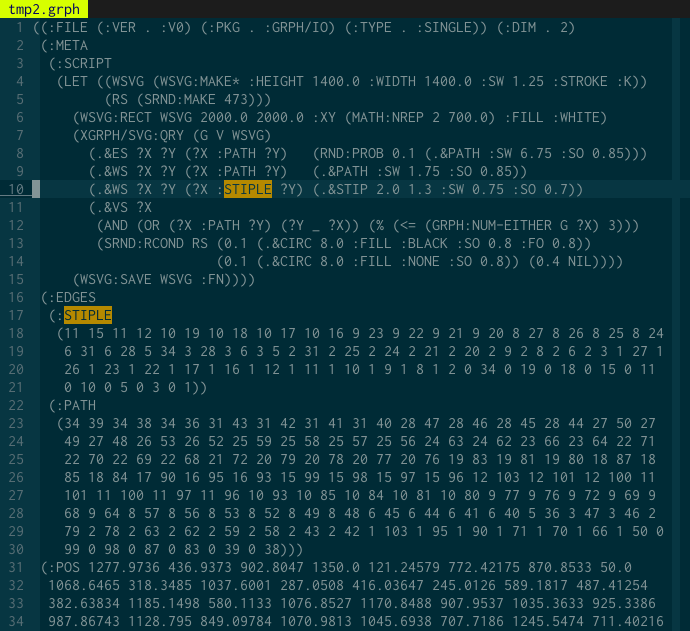
Obviously this might get more complicated for more realistic examples. But below is a screenshot from a complete .grph file for one of the illustrations in this post, and it should be quite recognizable.

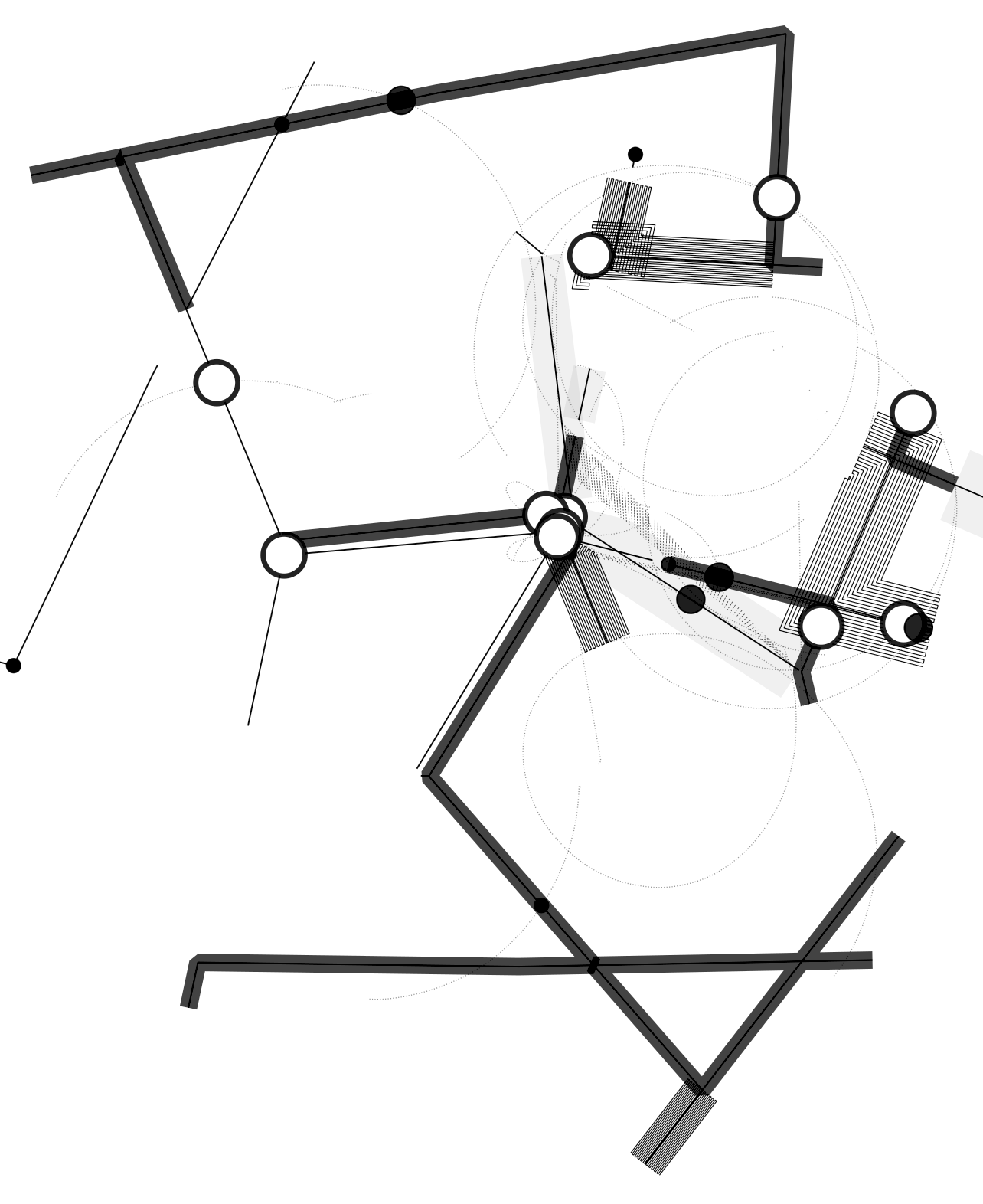
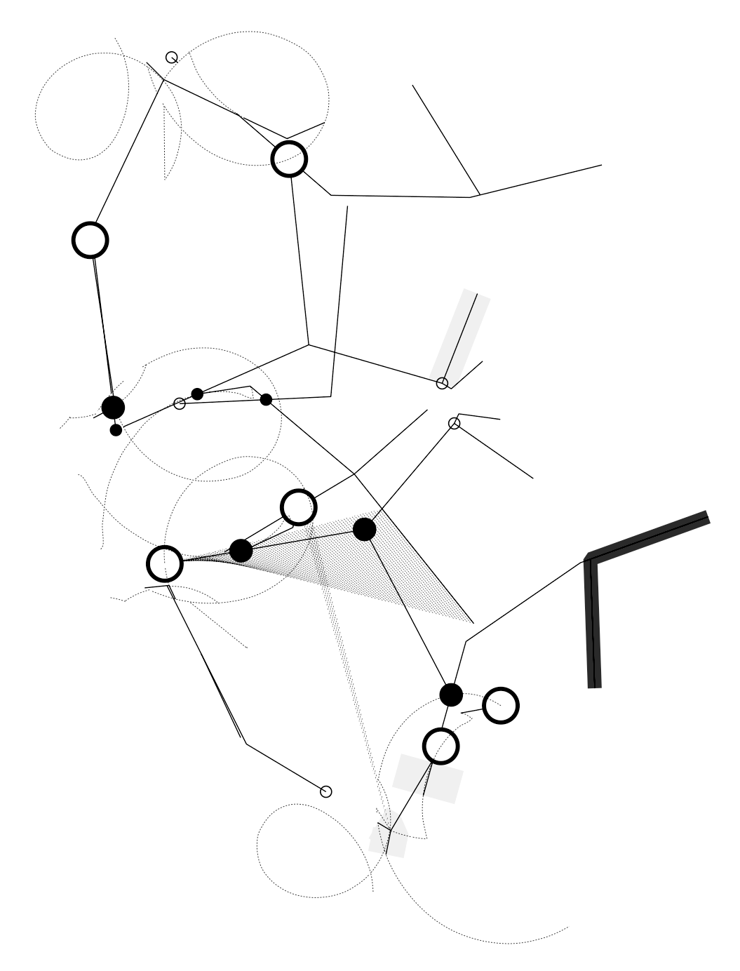
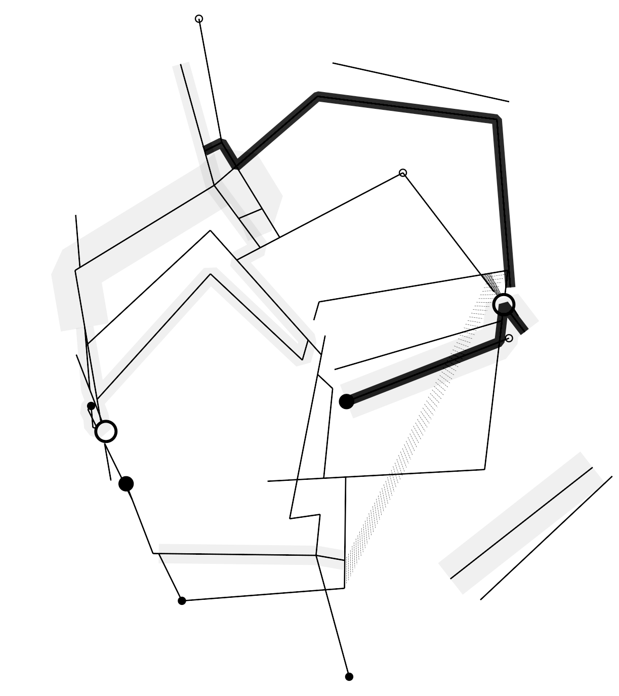
Out of interest I can also point out that the .grph files for the illustrations in this post are between 10-200 times smaller than the corresponding .svg. While containing sufficient information to create the identical .svg again; or draw it in a different manner.

The utility of this code in particular is pretty marginal to anyone except me. But I hope it serves as an interesting example of how Lisp (macros) can be used to do useful things. Things that—at the very least—would be more cumbersome to achieve in many other languages.

EDIT: In the next post I show how to implement a simplified version of the DSL.